Expert Tip: Geometric Non-linear Analysis Examples

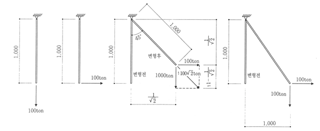
In the previous blog Geometric Nonlinearity Explained, various geometric nonlinear conditions are listed. To understand the differences between each non-linear theory, let’s consider a simple example as shown below. (Lee, Design, and Analysis of Suspension Bridges, 2001)

Figure 1. Example of a truss subject to vertical and horizontal loads. 

Consider a truss element, L = 1 m and the self-weight is Pv = 100 ton. Top end is supported by a pin support. Let’s calculate the displacement and axial force for given horizontal force Ph = 100 ton. Assume EA = ∞ to ignore the axial elongation.

• Linear Methods 

In the linear methods, this structure is unstable. We cannot analyze this structure.

• Linearized Finite Displacement Methods          

The horizontal stiffness is Kh = Pv/L = 100 ton/m and horizontal displacement is Δh = Ph/Kh = (100 ton) / (100 ton/m) = 1m. Truss axial force is 100 ton. Equilibnrium equation is formed for before-displaced condition.

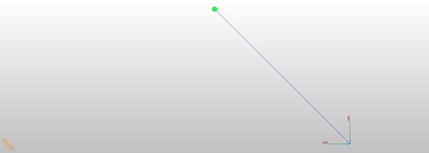
Figure 2. Deformed shape for Ph = 100 ton. See the Midas Civil file here 

• Finite Displacement Methods

For this example, same as linearized finite displacement methods. See the Midas Civil file here. 

• Large Displacement Methods

The truss axial force is 100√2 = 141.4 ton from force equilibrium after displaced. The displacements are Δh = 1/√2 = 0.7071 m and Δv = 1 – 1/√2 = 0.2929 m. 

For a given load Ph = ∞, Δh = Δv = 1 m ignoring axial elongation as expected. In other words, the truss shape is changed from vertical to horizontal due to infinite horizontal loads. This is a very simple example, but one of the extreme non-linear problems.

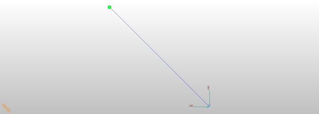
Figure 3. Deformed shape for Ph = 100 ton. See the Midas Civil file here.  

Figure 4. Deformed shape for Ph = ∞

• Discussion

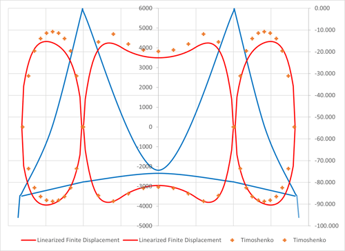
In the (linearized) finite displacement methods, the force equilibrium is considered for before-displaced conditions and we cannot consider the effects of axial stiffness, EA, and this is why the horizontal displacement Δh is larger than those from large displacement methods. Also, we cannot calculate vertical displacement Δv and the after-displaced element length is not correct.

In the large displacement methods, the total force Ph is applied without any divided load steps. In other words, the total load is assumed to be applied at once. This is applicable only to simple cases (and with a good solver) and normally we have to divide the loads into small load increases, like 0.1Ph.

The (linearized) finite displacement has been very well formulized we can expect the same solution from any commercial programs. However, the large displacement method has not, and every calculation procedure has its own assumptions and limitations. We may not need to fully understand the detailed calculation procedures, however, we have to understand the basic assumptions and limitations otherwise we may misunderstand the output.
Finally, in most bridge structures, the linearized finite displacement method gives very satisfactory results because the displacements are limited for serviceability.