Expert Tip: Why Not Solving Dynamic Problems Using Excel?

What is the Equilibrium Equation for Dynamic Problems? 

The equilibrium equation for any dynamic problem can be expressed as Eq (1).

Eq (1) is just an extension of a more familiar equilibrium equation for a static problem.

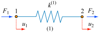
Figure 1. Representation of a simple static spring system. 

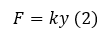
In Eq (2), F is the applied force, k is the stiffness, and y is the displacement. We know F and K, so we can calculate y. In other words, we have only one unknown y, so we can calculate y.

In Eq (1), F(t) is the applied force, k is the stiffness, and y(t) is the displacement just like in Eq (2). y(t) varies along time t because applied load F(t) varies along time t.

In Eq (1), m is mass and c is damping (whatever it means). y”(t) and y’(t) are the acceleration and velocity at time t. Now we have three unknowns, y”(t), y’(t), and y(t), looks like we will have a hard time solving Eq (1).

We know that acceleration y”(t) is derivative of velocity y’(t), and velocity y’(t) is derivative of displacement y(t). So if we know one of these, we can calculate the two others either by derivation or integration.

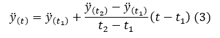
Let’s assume acceleration y”(t) varies linearly between t1 and t2. Then y”(t) can be defined as Eq (3).

Now we can calculate velocity y’(t) from integration.

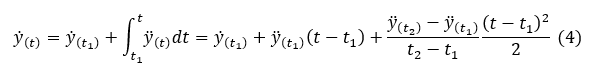
Velocity at time t2, y’(t2) is

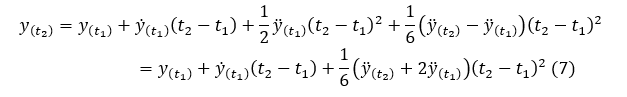
Now we can calculate displacement y(t) from integration.

Displacement at time t2, y(t2) is

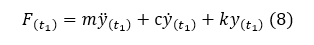
Now, we can calculation y”(t2) (and y’(t2), and y(t2)) if we knew y”(t1), y’(t1), and y(t1).
At time t1,

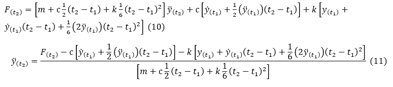
At time t2, from Eq (1), (5), and (7)

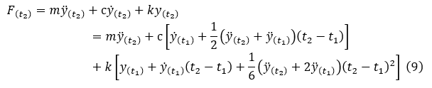
From Eq (9),

Let’s solve a simple problem:

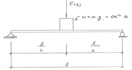
Figure 2. A mass sitting on a simply supported beam and is subjected to a time-dependent load F(t). 

Figure 3. The time-dependent function of the load F(t).

k = F/y = 48EI/L3 is given 2as000 lb/ft.

Damping C is given as 12.649 lb/(ft/sec).

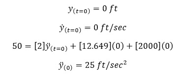
m = W/g = (64.4 lb)/(32.2 ft/sec2) = 2 lb/(ft/sec2)

When t1=0,

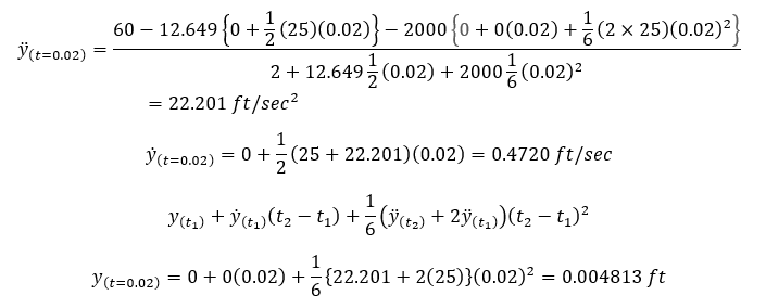
When t2=0.02,

When t=0.04,

Repeat these calculations as required. The summary is shown below,

Table 1. Dynamic Analysis (considering damping).

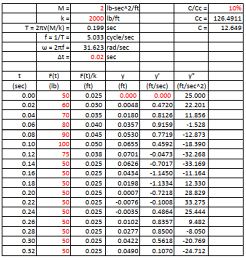
All structural dynamic systems contain damping to some degree, but the effect may not be significant if the load duration is short and only the maximum dynamic response is of interest. Also to find out the damping value itself is not an easy task.

The same analysis can be done easily through the same computational procedure.

Table 2. Dynamic Analysis (ignoring damping).

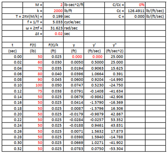
This method is rather simple, however gives very reasonable results. The only assumption that was introduced is, the acceleration varies linearly within a time step.

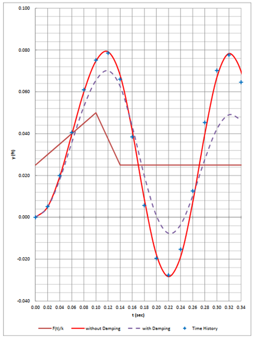
Figure 4. The plot of displacement y(t) against time t. With the maroon line representing the linear static response, the red line representing the dynamic response without considering damping, the purple dashed line representing the dynamic response with damping, and the blue crosses representing the time history analysis result from Midas Civil. 

The difference due to damping is around 10% in this example as shown in the graph. In the author’s view, these differences can be ignored in most practical problems because the precision of damping value itself is not that high. The time history analysis results from MIDAS (not considering damping) are also shown. The two results match very well.

The excel file and Midas Civil file are attached. I encourage the readers to perform a time history analysis with damping and compare the results.